Hint

You can run this notebook in a live session with .

DEDT Lumi through ECMWF Polytope API

The EMCWF Polytope API now supports bespoke geometry definions in queries.

eodag supports this feature via de geom parameter for the dedt_lumi provider.

from eodag import EODataAccessGateway
import json

dag = EODataAccessGateway()

result = dag.search(
    provider="dedt_lumi",
    start="2021-01-01",
    productType="DT_CLIMATE_ADAPTATION",
    geom={'lonmin': 22, 'latmin': 18, 'lonmax': 37, 'latmax': 45},
)

result

SearchResult (1)

0  EOProduct(id=DT_CLIMATE_ADAPTATION_ORDERABLE_c9ed022bda4820372d1eda2f3105d47a8a6396ad, provider=dedt_lumi) EOProduct provider: 'dedt_lumi', product_type: 'DT_CLIMATE_ADAPTATION', properties["id"]: 'DT_CLIMATE_ADAPTATION_ORDERABLE_c9ed022bda4820372d1eda2f3105d47a8a6396ad', properties["startTimeFromAscendingNode"]: '2021-01-01T00:00:00.000Z', properties["completionTimeFromAscendingNode"]: '2021-01-01T00:00:00.000Z', properties: (30) { keywords: 'DT,DE,LUMI,Destination-Earth,Digital-Twin,Climate,Change,Adaptation', license: 'other', title: 'DT_CLIMATE_ADAPTATION_ORDERABLE_c9ed022bda4820372d1eda2f3105d47a8a6396ad', missionStartDate: '2020-01-01T00:00:00Z', _id: 'DT_CLIMATE_ADAPTATION', productType: 'climate-dt', ecmwf:resolution: 'high', startTimeFromAscendingNode: '2021-01-01T00:00:00.000Z', completionTimeFromAscendingNode: '2021-01-01T00:00:00.000Z', id: 'DT_CLIMATE_ADAPTATION_ORDERABLE_c9ed022bda4820372d1eda2f3105d47a8a6396ad', ecmwf:time: '0000', ecmwf:param: '134/165/166', ecmwf:feature: { 'shape': [[18.0 , 22.0 ] , [45.0 , 22.0 ] , [45.0 , 37.0 ] , [18.0 , 37.0 ] , [18.0 , 22.0 ] ] , 'type': 'polygon' }, ecmwf:activity: 'ScenarioMIP', ecmwf:levtype: 'sfc', ecmwf:expver: '0001', ecmwf:realization: 1, ecmwf:generation: 1, ecmwf:date: '20210101/to/20210101', ecmwf:experiment: 'SSP3-7.0', ecmwf:class: 'd1', ecmwf:model: 'IFS-NEMO', ecmwf:stream: 'clte', ecmwf:dataset: 'climate-dt', ecmwf:type: 'fc', storageStatus: 'OFFLINE', defaultGeometry: 'POLYGON((180 -90, 180 90, -180 90, -180 -90, 180 -90))', qs: { 'activity': 'ScenarioMIP' , 'class': 'd1' , 'dataset': 'climate-dt' , 'date': '20210101/to/20210101' , 'experiment': 'SSP3-7.0' , 'expver': '0001' , 'feature': { 'shape': [[18.0 , 22.0 ] , [45.0 , 22.0 ] , [45.0 , 37.0 ] , [18.0 , 37.0 ] , [18.0 , 22.0 ] ] , 'type': 'polygon' } , 'generation': 1 , 'levtype': 'sfc' , 'model': 'IFS-NEMO' , 'param': '134/165/166' , 'realization': 1 , 'resolution': 'high' , 'stream': 'clte' , 'time': '0000' , 'type': 'fc' }, orderLink: 'https://polytope.lumi.apps.dte.destination-earth.eu/api/v1/requests/destination-earth?{"verb": "retrieve", "request": {"activity": "ScenarioMIP", "class": "d1", "dataset": "climate-dt", "date": "20210101/to/20210101", "experiment": "SSP3-7.0", "expver": "0001", "feature": {"shape": [[18.0, 22.0], [45.0, 22.0], [45.0, 37.0], [18.0, 37.0], [18.0, 22.0]], "type": "polygon"}, "generation": 1, "levtype": "sfc", "model": "IFS-NEMO", "param": "134/165/166", "realization": 1, "resolution": "high", "stream": "clte", "time": "0000", "type": "fc"} }', _dc_qs: '%7B%22activity%22%3A+%22ScenarioMIP%22%2C+%22class%22%3A+%22d1%22%2C+%22dataset%22%3A+%22climate-dt%22%2C+%22date%22%3A+%2220210101%2Fto%2F20210101%22%2C+%22experiment%22%3A+%22SSP3-7.0%22%2C+%22expver%22%3A+%220001%22%2C+%22feature%22%3A+%7B%22shape%22%3A+%5B%5B18.0%2C+22.0%5D%2C+%5B45.0%2C+22.0%5D%2C+%5B45.0%2C+37.0%5D%2C+%5B18.0%2C+37.0%5D%2C+%5B18.0%2C+22.0%5D%5D%2C+%22type%22%3A+%22polygon%22%7D%2C+%22generation%22%3A+1%2C+%22levtype%22%3A+%22sfc%22%2C+%22model%22%3A+%22IFS-NEMO%22%2C+%22param%22%3A+%22134%2F165%2F166%22%2C+%22realization%22%3A+1%2C+%22resolution%22%3A+%22high%22%2C+%22stream%22%3A+%22clte%22%2C+%22time%22%3A+%220000%22%2C+%22type%22%3A+%22fc%22%7D', } assets: (0) geometry

Let’s download this product and check its data.

path = result[0].download(output_dir='/tmp')

!tree {path}

[Retry #7] Waiting 11.595347s until next order status check (retry every 0.2' for 10')

/tmp/DT_CLIMATE_ADAPTATION_a6764da7-9c5c-472d-a884-e965d127423f
└── DT_CLIMATE_ADAPTATION_a6764da7-9c5c-472d-a884-e965d127423f.covjson

1 directory, 1 file

When requesting a RoI, ECMWF Polytope will generate a covjson file.

To plot it, we are going to load it into an xarray dataset.

import os
import json
from covjsonkit.api import Covjsonkit

import matplotlib.pyplot as plt
import cartopy.crs as ccrs
import cartopy.feature as cfeature

cov_json_path = os.path.join(path, os.listdir(path)[0])

with open(cov_json_path) as f:
    covjson = json.load(f)

# Load CovJson using covjsonkit into an xarray
decoder = Covjsonkit().decode(covjson)
ds = decoder.to_xarray()

ds

<xarray.Dataset> Size: 6MB
Dimensions:    (datetimes: 1, number: 1, steps: 1, points: 104351)
Coordinates:
  * datetimes  (datetimes) <U20 80B '2021-01-01 00:00:00Z'
  * number     (number) int64 8B 0
  * steps      (steps) int64 8B 0
  * points     (points) int64 835kB 0 1 2 3 4 ... 104347 104348 104349 104350
    latitude   (points) float64 835kB 18.01 18.01 18.01 ... 44.99 44.99 44.99
    longitude  (points) float64 835kB 22.06 22.15 22.24 ... 36.8 36.89 36.98
    levelist   (points) float64 835kB 0.0 0.0 0.0 0.0 0.0 ... 0.0 0.0 0.0 0.0
Data variables:
    sp         (datetimes, number, steps, points) float64 835kB 9.549e+04 ......
    10u        (datetimes, number, steps, points) float64 835kB -5.133 ... 4.259
    10v        (datetimes, number, steps, points) float64 835kB -0.9033 ... 8...
Attributes: (12/15)
    activity:     scenariomip
    class:        d1
    dataset:      climate-dt
    experiment:   ssp3-7.0
    expver:       0001
    generation:   1
    ...           ...
    resolution:   high
    stream:       clte
    type:         fc
    number:       0
    step:         0
    date:         2021-01-01 00:00:00Z

xarray.Dataset

• Dimensions:
  • datetimes: 1
  • number: 1
  • steps: 1
  • points: 104351
• Coordinates: (7)
  • datetimes
    (datetimes)
    <U20
    '2021-01-01 00:00:00Z'

    array(['2021-01-01 00:00:00Z'], dtype='<U20')

  • number
    (number)
    int64
    0

    array([0])

  • steps
    (steps)
    int64
    0

    array([0])

  • points
    (points)
    int64
    0 1 2 3 ... 104348 104349 104350

    array([     0,      1,      2, ..., 104348, 104349, 104350], shape=(104351,))

  • latitude
    (points)
    float64
    18.01 18.01 18.01 ... 44.99 44.99

    array([18.01372403, 18.01372403, 18.01372403, ..., 44.99388015,
           44.99388015, 44.99388015], shape=(104351,))

  • longitude
    (points)
    float64
    22.06 22.15 22.24 ... 36.89 36.98

    array([22.06054688, 22.1484375 , 22.23632812, ..., 36.796875  ,
           36.890625  , 36.984375  ], shape=(104351,))

  • levelist
    (points)
    float64
    0.0 0.0 0.0 0.0 ... 0.0 0.0 0.0 0.0

    array([0., 0., 0., ..., 0., 0., 0.], shape=(104351,))

• Data variables: (3)
  • sp
    (datetimes, number, steps, points)
    float64
    9.549e+04 9.544e+04 ... 1.02e+05

    type :

    Parameter

    units :

    Pa

    long_name :

    sp

    array([[[[ 95489.52734375,  95442.27734375,  95363.0703125 , ...,
              101980.1953125 , 101970.14453125, 101996.37109375]]]],
          shape=(1, 1, 1, 104351))

  • 10u
    (datetimes, number, steps, points)
    float64
    -5.133 -5.366 ... 4.405 4.259

    type :

    Parameter

    units :

    m s**-1

    long_name :

    10u

    array([[[[-5.13264847, -5.36615753, -5.79761124, ...,  4.40535355,
               4.40521622,  4.25865555]]]], shape=(1, 1, 1, 104351))

  • 10v
    (datetimes, number, steps, points)
    float64
    -0.9033 -0.7706 ... 8.582 8.549

    type :

    Parameter

    units :

    m s**-1

    long_name :

    10v

    array([[[[-0.90330315, -0.77064323, -0.49776649, ...,  8.42875862,
               8.58184242,  8.54909325]]]], shape=(1, 1, 1, 104351))

• Indexes: (4)
  • datetimes
    PandasIndex

    PandasIndex(Index(['2021-01-01 00:00:00Z'], dtype='object', name='datetimes'))

  • number
    PandasIndex

    PandasIndex(Index([0], dtype='int64', name='number'))

  • steps
    PandasIndex

    PandasIndex(Index([0], dtype='int64', name='steps'))

  • points
    PandasIndex

    PandasIndex(Index([     0,      1,      2,      3,      4,      5,      6,      7,      8,
                9,
           ...
           104341, 104342, 104343, 104344, 104345, 104346, 104347, 104348, 104349,
           104350],
          dtype='int64', name='points', length=104351))

• Attributes: (15)

  activity :

  scenariomip

  class :

  d1

  dataset :

  climate-dt

  experiment :

  ssp3-7.0

  expver :

  0001

  generation :

  1

  levtype :

  sfc

  model :

  ifs-nemo

  realization :

  1

  resolution :

  high

  stream :

  clte

  type :

  fc

  number :

  0

  step :

  0

  date :

  2021-01-01 00:00:00Z

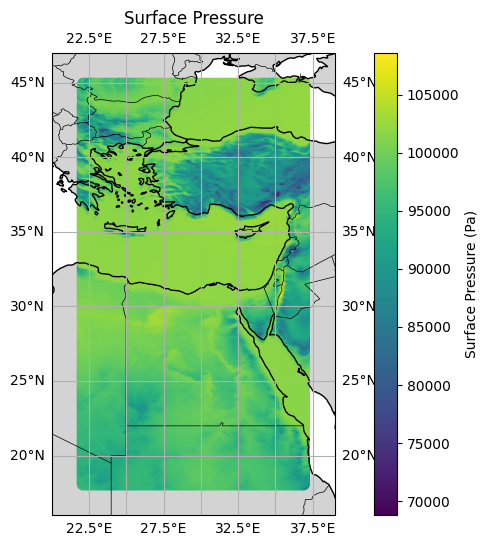
# Extracting sp variable from dataset
# Data in the original covjson is organize in points rather than lat/lon variables
# so we plot as scatter.

sp = ds['sp'].isel(datetimes=0, number=0, steps=0).values
lats = ds['latitude'].values
lons = ds['longitude'].values

fig = plt.figure(figsize=(10,6))
ax = plt.axes(projection=ccrs.PlateCarree())

# Add features
ax.coastlines()
ax.gridlines(draw_labels=True)
ax.add_feature(cfeature.BORDERS, linewidth=0.5)
ax.add_feature(cfeature.LAND, facecolor='lightgray')

sc = ax.scatter(lons, lats, c=sp, s=40, cmap='viridis',
                transform=ccrs.PlateCarree())

plt.colorbar(sc, orientation='vertical', label='Surface Pressure (Pa)')

margin = 2
ax.set_extent([
    lons.min()-margin, lons.max()+margin,
    lats.min()-margin, lats.max()+margin
], crs=ccrs.PlateCarree())

plt.title("Surface Pressure")
plt.show()